Now that we have established the basics of vector analysis, it is time to start our journey on Electromagnetic (EM) field theory. We start at first with Coulomb’s law and then move on to the other important laws before deriving Maxwell’s equations.

What is Coulomb’s law?

Coulomb’s law was experimentally investigated by Colonel Charles Coulomb of French army engineers. This law states that the force between two point charges (very small compared to the distance by which they are separated) is directly proportional to their individual charge (Q) and inversely proportional to the square of the distance (R) between them. Coulomb’s law can be mathematically depicted by the following formulation.

\[\overrightarrow{F}=k\frac{Q_1 Q_2}{R^2}\]

where k is dependent on the permittivity (that is linked to the refractive index of the material) of the free space as shown below.

\[k=\frac{1}{4 \pi \epsilon_o}\]

Therefore, Coulomb’s law for two point charges in free space is given by Eq. 1.

\[\overrightarrow{F}=\frac{Q_1 Q_2}{4 \pi \epsilon_o R^2}\hspace{1cm}(1)\]

Since Coulomb’s law defines force, it has units of N (newtons). The permittivity of free space is 8.85418782×10^-12 and has units of C²/Nm² or F/m. The value of k as a whole is 8.987551785×10⁹ or sometimes approximated as 9×10⁹. Adding our discussion on vector analysis, the vector form of Coulomb’s law for two point charges Q₁ (at position r₁) and Q₂ (at position r₂) separated by a distance r₁₂ is given by Eq. 2.

\[\overrightarrow{F}_{1\rightarrow 2}=\frac{Q_1 Q_2}{4 \pi \epsilon_o r_{12}^2}\overrightarrow{a_{12}}\hspace{1cm}(2)\]

The term r₁₂ is defined by the position of two point charges and is given as r₁₂ = r₂ – r₁. The term a₁₂ is the unit vector along the distance r₁₂. The Eq. 2 represents the force exerted by Q₁ on Q₂. In order to evaluate a simple problem using this formula, let us consider an example.

Example 1

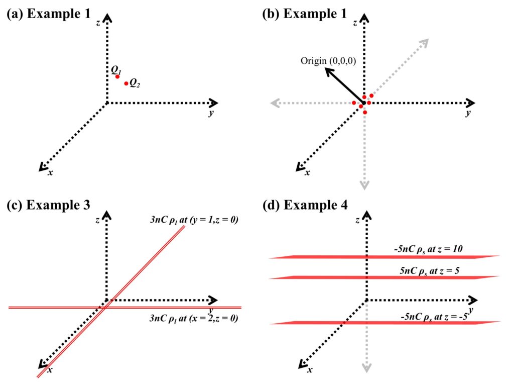
We have two point charges Q₁=2 μC and Q₂=15 μC, located at points (2,3,6) and (2,6,5), respectively. Let’s find the force exerted by Q₁ on Q₂ and vice versa. [Figure 1(a)]

1. First calculate r₁₂.

\[\overrightarrow{r_{12}}=\overrightarrow{r_2} – \overrightarrow{r_1}\]\[=(2-2)\overrightarrow{a_x}+(6-3)\overrightarrow{a_x}+(5-6)\overrightarrow{a_z}\]\[=3\overrightarrow{a_x}-\overrightarrow{a_z}\]

Similarly, r₂₁ will be.

\[\overrightarrow{r_{21}}=\overrightarrow{r_1} – \overrightarrow{r_2}\]\[=-3\overrightarrow{a_x}+\overrightarrow{a_z}\]

2. Calculate the distance r₁₂ which will be the same for r₂₁.

\[|\overrightarrow{r_{12}}|=\sqrt{10}\]

3. Calculate the unit vector.

\[\overrightarrow{a_{12}}=\frac{3\overrightarrow{a_x}-\overrightarrow{a_z}}{\sqrt{10}}\]\[=-\overrightarrow{a_{21}}\]

4. Calculate the force exerted by the charge by utilizing Eq. 2.

\[\overrightarrow{F}_{1\rightarrow 2}=\frac{Q_1 Q_2}{4 \pi \epsilon_o r_{12}^2}\overrightarrow{a_{12}}\]\[=\frac{2\times 15}{40 \pi \epsilon_o}\times \frac{3\overrightarrow{a_x}-\overrightarrow{a_z}}{\sqrt{10}}\]\[=0.026963(3\overrightarrow{a_x}-\overrightarrow{a_z}) N\]

Similarly, force on charge Q₁ can be calculated as.

\[\overrightarrow{F}_{2\rightarrow 1}=0.026963(-3\overrightarrow{a_x}+\overrightarrow{a_z}) N\]\[=-\overrightarrow{F}_{1\rightarrow 2}\]

Electric field intensity

After calculating force on charges, now consider a situation where one point charge is at a fixed position and the other point charge is moved around the fixed charge. The moving or test charge will experience a force when the fixed charge is in affinity. This force per unit charge that the test charge experiences is called an electric field intensity, given by E, and having units of N/C or more commonly known as V/m. The electric field from positive charges flows out while the electric field from negative charges flows in an inward direction, as shown in Fig. 2. Two positive charges or two negative charges repel each other and two charges with different charges attract each other such that field from positive charges flows toward negative charges.

Figure 2: Depiction of electric fields from positive and negative charges.

In mathematical form, electric field intensity for charge Q₁ and test charge Q_t is given by Eq. 3.

\[\overrightarrow{E}_{1\rightarrow t}=\frac{\overrightarrow{F}_{1\rightarrow t}}{Q_t}\]\[\overrightarrow{E}_{1\rightarrow t}=\frac{Q_1}{4 \pi \epsilon_o r_{12}^2}\overrightarrow{a_{1t}}\hspace{1cm}(3)\]

Since the force between two charges is linear, the electric field due to many charges (n) at point r can be calculated by the summation of all the electric fields due to all the charges. The Eq. 3 can then be modified to Eq. 4.

\[\overrightarrow{E(r)}=\frac{Q_1}{4 \pi \epsilon_o r_{1r}^2}\overrightarrow{a_{1r}}+\frac{Q_2}{4 \pi \epsilon_o r_{2r}^2}\overrightarrow{a_{2r}}\]\[+\cdots+\frac{Q_n}{4 \pi \epsilon_o r_{nr}^2}\overrightarrow{a_{nr}}\]\[\overrightarrow{E(r)}=\sum_{m=1}^{n}\frac{Q_m}{4 \pi \epsilon_o r_{mr}^2}\overrightarrow{a_{nr}}\]

\[\overrightarrow{E(r)}=\sum_{m=1}^{n}\frac{Q_m}{4 \pi \epsilon_o |r-r_m|^2}\frac{(r-r_m)}{|r-r_m|}\hspace{1cm}(4)\]

Example 2

Let us take an example of 6 equal charges of 5 nC placed at (1,0,0), (-2,0,0), (0,1,0), (0,-2,0), (0,0,1), and (0,0,-2). We can calculate the electric field at (0,0,0) by summation of all electric fields by individual charges. [Figure 1(b)]

The vector (r–r_m) for all the charges will be –a_x (distance of 1), 2a_x (distance of 2), –a_y (distance of 1), 2a_y (distance of 2), –a_z (distance of 1), and 2a_z (distance of 2). The term k (1/4πε_o) multiplied by 5 nC is approximately 44.94 V.m. The total electric field at point (0,0,0) is given as follows.

\[\overrightarrow{E}=-44.94 \overrightarrow{a_x}+5.62 \overrightarrow{a_x}-44.94 \overrightarrow{a_y}+5.62 \overrightarrow{a_y}\]\[-44.94 \overrightarrow{a_z}+5.62 \overrightarrow{a_z}\]\[\overrightarrow{E}=-39.32\overrightarrow{a_x}-39.32\overrightarrow{a_y}-39.32\overrightarrow{a_z} V/m\]

Volume charge, line charge and sheet charge

The volume, line, and sheet charge distributions are represented by ρ_v, ρ_l, and ρ_s, respectively. The units of ρ_v, ρ_l, and ρ_s are C/m³,C/m, and C/m². The total charge enclosed in a volume is given by Eq. 5.

\[Q=\int_{vol}\rho_v dv\]

The Eq. 4 can be modified a little to calculate the electric field intensity due to many volume charges by Eq. 5.

\[\overrightarrow{E(r)}=\int_{vol}\frac{\rho_v(r_m) dv}{4 \pi \epsilon_o |r-r_m|^2}\frac{(r-r_m)}{|r-r_m|}\hspace{1cm}(4)\]

A line charge is a line of charges that extends to infinity to make a line. For example, if we consider the line charge to be at origin and the line extends to both positive and negative infinity along z-axis, it can be observed the electric field would not vary if we move along φ in cylindrical coordinates. Moreover, along z-axis there will not be any change in the electric field intensity as well because the field intensities due to two point in opposite directions will cancel each other. The only thing that will vary the electric field intensity is ρ. In order to calculate the field at an arbitrary point ρ due to a point in z-axis z, we can take Q charge as ρ_ldz .

\[d\overrightarrow{E}=\frac{\rho_l dz (r-r_m)}{4\pi\epsilon_o|r-r_m|^3}\] \[r=\rho\overrightarrow{a_\rho}\] \[r_m=z\overrightarrow{a_z}\] \[r-r_m=\rho\overrightarrow{a_\rho}-z\overrightarrow{a_z}\] \[d\overrightarrow{E}=\frac{\rho_l dz (\rho\overrightarrow{a_\rho}-z\overrightarrow{a_z})}{4\pi\epsilon_o(\rho^2+z^2)^\frac{3}{2}}\]

Since we discussed that the z component will be zero.

\[d\overrightarrow{E}=\frac{\rho_l \rho dz }{4\pi\epsilon_o(\rho^2+z^2)^\frac{3}{2}}\]

Integrating the above expression with variable change as follows.

\[z=\rho \tan \theta\] \[dz=\rho \sec^2\theta d\theta\] \[E=\frac{\rho_l \rho^2}{4\pi\epsilon_o\rho^3 }\int_{-\infty}^{\infty} \frac{\sec^2\theta d\theta }{(1+ \tan^2 \theta)^\frac{3}{2}}\hspace{0.5cm}(5)\]

\[1+\tan^2 \theta=\sec^2 \theta\]

the expression in Eq. 5 can be written as follows.

\[E=\frac{\rho_l}{4\pi\epsilon_o\rho }\int_{-\infty}^{\infty} \cos \theta\] \[E=\frac{\rho_l }{4\pi\epsilon_o\rho}|\sin \theta|_{-\infty}^{\infty}\hspace{0.5cm}(6)\]

From here we can employ two methods. Method 1 will incorporate the variables back into Eq. 6 and then solve the equation. In Method 2 the limits of the above expression will be changed to deal with the equation in θ.

Method 1.

From variable change, we can find the value of sinθ.

\[z=\rho\tan\theta\] \[\frac{z}{\rho}=\frac{\sin\theta}{\cos\theta}\] \[\frac{z^2}{\rho^2}=\frac{\sin^2\theta}{\cos^2\theta}\] \[\frac{z^2}{\rho^2}=\frac{\sin^2\theta}{\cos^2\theta}+\frac{\cos^2\theta}{\cos^2\theta}-1\] \[\frac{z^2}{\rho^2}+1=\frac{1}{\cos^2\theta}\] \[\frac{\rho^2+z^2}{\rho^2}=\frac{1}{\cos^2\theta}\] \[\frac{\rho^2}{\rho^2+z^2}=\cos^2\theta\] \[\frac{\rho^2}{\rho^2+z^2}=1-\sin^2\theta\] \[\sin^2\theta=1-\frac{\rho^2}{\rho^2+z^2}\] \[\sin^2\theta=\frac{z^2}{\rho^2+z^2}\] \[\sin\theta=\frac{z}{\sqrt{\rho^2+z^2}}\]

Substituting the value of sinθ in Eq. 6.

\[E=\frac{\rho_l }{4\pi\epsilon_o\rho}\left| \begin{array}{cc} \frac{z}{\sqrt{\rho^2+z^2}} \end{array} \right|_{-\infty}^{\infty}\]

which comes out to be

\[E=\frac{\rho_l }{2\pi\epsilon_o\rho}\hspace{0.5cm}(7)\]

Method 2.

The value of θ is π/2 for +∞ and it is -π/2 for +∞. Resolving Eq. 6 for θ with limits of π/2 and -π/2.

\[E=\frac{\rho_l }{4\pi\epsilon_o\rho}|\sin \theta|_{-\pi/2}^{\pi/2}\] \[E=\frac{\rho_l }{4\pi\epsilon_o\rho}(1-(-1))\] \[E=\frac{\rho_l }{2\pi\epsilon_o\rho}\hspace{0.5cm}(7)\]

The Eq. 7 gives the electric field intensity of a line charge and reveals that the electric field intensity decreases as the reference moves away from the line charge. But this effect is not as pronounced as the decrease in the electric field from a point source. In vector form, the Eq. 7 can be written as Eq. 8.

\[\overrightarrow{E}=\frac{\rho_l }{2\pi\epsilon_o\rho}\overrightarrow{a_\rho}\hspace{0.5cm}(8)\]

Example 3

Let’s take two line charges with a charge of 3nC/m placed at y=1,z=0 (parallel to the x-axis), and x=2,z=0 (parallel to the y-axis) and find the electric field contribution of these line charges at points P(0,0,5) and Q(3,4,5). [Figure 1(c)]

The line charges will contribute to the electric field on the other two axes than they are situated at.

For line charge at y=1.

\[\overrightarrow{E}=\frac{\rho_l [(y-1)\overrightarrow{a_y}+(z-0)\overrightarrow{a_z}]}{2\pi\epsilon_o[(y-1)^2+(z-0)^2]}\]

For line charge at x=2.

\[\overrightarrow{E}=\frac{\rho_l [(x-2)\overrightarrow{a_x}+(z-0)\overrightarrow{a_z}]}{2\pi\epsilon_o[(x-2)^2+(z-0)^2]}\]

Electric field contributions at point P.

\[\overrightarrow{E}=\frac{3nC [-\overrightarrow{a_y}+5\overrightarrow{a_z}]}{52\pi\epsilon_o}+\frac{3nC [-2\overrightarrow{a_x}+5\overrightarrow{a_z}]}{60\pi\epsilon_o}\] \[=-2.08\overrightarrow{a_y}+10.38\overrightarrow{a_z}-3.6\overrightarrow{a_x}+9\overrightarrow{a_z}\] \[=-3.6\overrightarrow{a_x}-2.08\overrightarrow{a_y}+19.38\overrightarrow{a_z} V/m\]

Electric field contributions at point Q.

\[\overrightarrow{E}=\frac{3nC [3\overrightarrow{a_y}+5\overrightarrow{a_z}]}{52\pi\epsilon_o}+\frac{3nC [\overrightarrow{a_x}+5\overrightarrow{a_z}]}{60\pi\epsilon_o}\] \[=6.24\overrightarrow{a_y}+10.38\overrightarrow{a_z}+1.8\overrightarrow{a_x}+9\overrightarrow{a_z}\] \[=1.8\overrightarrow{a_x}+6.24\overrightarrow{a_y}+19.38\overrightarrow{a_z} V/m\]

For sheet charge ρ_s, we can observe that it is an integral of line charge which had an infinite charge on a single line in an axis. The sheet of charge will have a charge on an infinite sheet in two dimensions. Therefore, the sheet charge can be represented by the following expression if the line charge was considered to be on the z-axis.

\[\rho_l=\rho_s dy\]

We can substitute this value in Eq. 8. Moreover, since we are considering sheet of charge as line charge which is infinitely varying over y-dimension, we can see that there will be no contribution of z in electric field intensity. The distance from any line charge to any arbitrary test point on x-axis will have a distance of R=ρ. The unit vector in the direction of the sheet charge will be cosθ.

\[R=\sqrt{x^2 +y^2}\] \[dE_x=\frac{\rho_s dy}{2\pi\epsilon_o\sqrt{x^2 +y^2}}\cos\theta\]

cosθ can be written as x/R.

\[dE_x=\frac{\rho_s x dy}{2\pi\epsilon_o (x^2 +y^2)}\]

Integrating to combine electric field from all line charges to make a sheet charge.

\[E_x=\frac{\rho_s}{2\pi\epsilon_o}\int_{-\infty}^{\infty}\frac{x dy}{ (x^2 +y^2)}\] \[E_x=\frac{\rho_s}{2\pi\epsilon_o}\left| \begin{array}{cc} \tan^{-1}\frac{y}{ x} \end{array} \right|_{-\infty}^{\infty}\] \[E_x=\frac{\rho_s}{2\pi\epsilon_o}\int_{-\infty}^{\infty}\frac{x dy}{ (x^2 +y^2)}\] \[E_x=\frac{\rho_s}{2\pi\epsilon_o}(\frac{\pi}{2}-(-\frac{\pi}{2}))\] \[E_x=\frac{\rho_s}{2\epsilon_o}\hspace{0.5cm}(9)\]

In vector form, the electric field due to the sheet of charge can be written as follows.

\[E_x=\frac{\rho_s}{2\epsilon_o}\overrightarrow{a_N}\hspace{0.5cm}(10)\]

where a_N is a unit vector perpendicular to the sheet of charge.

Example 4

Let’s take three sheets of charge. The first sheet has a charge of -5nC/m² each, placed at z=-5, the second sheet has a charge of 5nC/m² and is placed at z=5, and the last sheet has a charge of -5nC/m² and is placed at z=10. We need to find the electric field intensity at points A(0,0,-8), B(0,0,-3), C(0,0,2), D(0,0,7) and E(0,0,12). [Figure 1(d)]

Electric field intensity at point A.

\[\overrightarrow{E}=\frac{-5nC}{2\epsilon_o}\frac{(-8-(-5))\overrightarrow{a_z}}{\sqrt{-8+5}^2}-\frac{5nC}{2\epsilon_o}\overrightarrow{a_z}-\frac{5nC}{2\epsilon_o}\overrightarrow{a_z}\] \[=564\overrightarrow{a_z} V/m\]

Electric field intensity at point B.

\[\overrightarrow{E}=-\frac{5nC}{2\epsilon_o}\overrightarrow{a_z}-\frac{5nC}{2\epsilon_o}\overrightarrow{a_z}+\frac{5nC}{2\epsilon_o}\overrightarrow{a_z}\] \[=-564\overrightarrow{a_z} V/m\]

Electric field intensity at point C.

\[\overrightarrow{E}=\frac{5nC}{2\epsilon_o}\overrightarrow{a_z}-\frac{5nC}{2\epsilon_o}\overrightarrow{a_z}+\frac{5nC}{2\epsilon_o}\overrightarrow{a_z}\] \[=564\overrightarrow{a_z} V/m\]

Electric field intensity at point D.

\[\overrightarrow{E}=-\frac{5nC}{2\epsilon_o}\overrightarrow{a_z}+\frac{5nC}{2\epsilon_o}\overrightarrow{a_z}+\frac{5nC}{2\epsilon_o}\overrightarrow{a_z}\] \[=564\overrightarrow{a_z} V/m\]

Electric field intensity at point E.

\[\overrightarrow{E}=-\frac{5nC}{2\epsilon_o}\overrightarrow{a_z}+\frac{5nC}{2\epsilon_o}\overrightarrow{a_z}-\frac{5nC}{2\epsilon_o}\overrightarrow{a_z}\] \[=-564\overrightarrow{a_z} V/m\]

This concludes our discussion on Coulomb’s law and electric field intensity.