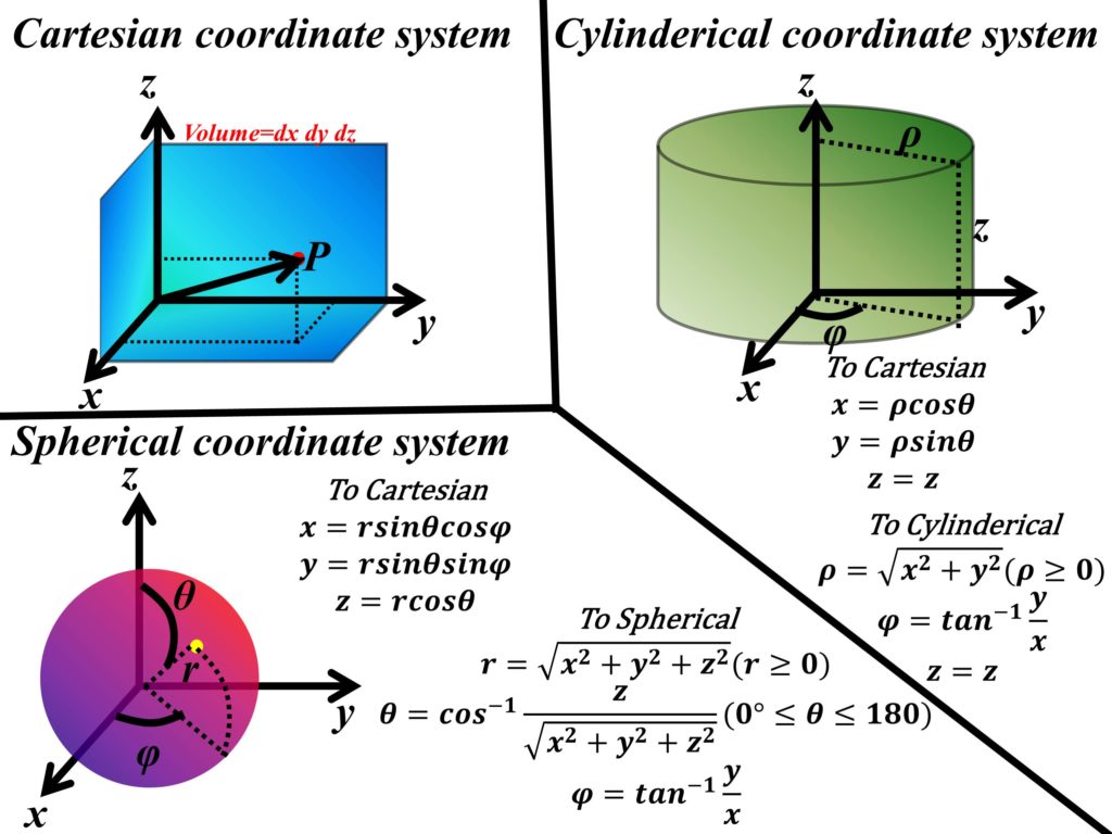
The streamlines from charges in the previous topic of “Coulomb’s law and electric field intensity” are actually not physically present or visually observable, but when these streamlines are drawn, they become a helpful tool to represent the presence of something. The term of electric flux also shows what the streamlines show, the presence of an electric field.

Electric flux and electric flux density

Michael Faraday carried out experiments using two concentric metallic spheres, that were able to firmly fit together. These two spheres were separated by a dielectric medium. The inner metallic sphere was given a quantifiable charge, and the outer sphere was grounded to remove any stray charge. The experiment revealed that the charge on the outer sphere (radius b) was equal to the charge given to the inner sphere (radius a), and it was therefore concluded that there was some sort of displacement of the inner sphere charge to the outer sphere. This phenomenon of displacement of electric charges is known as electric flux and is sometimes also referred to as displacement flux. In terms of streamlines, which also represent the flux, the electric flux is the number of electric field lines from a charge that intersect a surface.

It was also observed that a large charge of the inner sphere will yield a corresponding larger charge on the outer sphere. Therefore, electric flux (ψ) is proportional to the charge enclosed (Q) in the surface and the constant of proportionality is 1. In mathematical form, this can be mathematically represented by Eq. 1.

\[\psi=Q\hspace{1.5cm}(1)\]

If we continue to picture a sphere, the charges or electric flux produced by the inner sphere will be uniformly distributed on the surface. And similarly, the same will happen for the outer sphere. The surface area of a sphere is 4πr², and if we consider the radii of the inner sphere as a and the outer sphere as b, we will get the following expressions, which represent electric flux density (D) shown in Fig. 1(a).

\[\overrightarrow{D}=\frac{Q}{4\pi a^2}\overrightarrow{a_r}\hspace{0.5cm}inner\hspace{0.1cm}sphere\] \[\overrightarrow{D}=\frac{Q}{4\pi b^2}\overrightarrow{a_r}\hspace{0.5cm}outer\hspace{0.1cm}sphere\]

Figure 1: (a) Depiction of electric flux density (D). (b) Example 1: Calculating D at different ρ. (c) Example 2: Calculating ψ. (d) Example 3: Calculating electric flux density due to a point charge, line charge and sheet charge.

This shows that electric flux density (D) is the electric field lines that are passing through a surface area. It represents the strength of the electric field. The D of any other point in between two metallic spheres is represented by the following Eq. 2.

\[\overrightarrow{D}=\frac{Q}{4\pi r^2}\overrightarrow{a_r}\hspace{1cm}(2)\]

Similarly, the electric field intensity in free space is given by the following Eq. 3.

\[\overrightarrow{E}=\frac{Q}{4\pi \epsilon_o r^2}\overrightarrow{a_r}\hspace{1cm}(3)\]

From Eqs. 2 and 3, it can be observed that in free space.

\[\overrightarrow{D}=\epsilon_o\overrightarrow{E}\hspace{1cm}(4)\]

For a general volume charge, the electric field in free space can be written as follows.

\[\overrightarrow{E}=\frac{\rho_v dv}{4\pi \epsilon_o R^2}\overrightarrow{a_r}\hspace{1cm}(5)\]

Similarly, the ψ density will be given by the following Eq. 5.

\[\overrightarrow{D}=\frac{\rho_v dv}{4\pi R^2}\overrightarrow{a_r}\hspace{1cm}(5)\]

Example 1

If we have a line charge placed along the z-axis with a charge of 6 μC/m, find the D at ρ=3 and ρ=5 (shown in Fig 1(b)).

From our previous discussion.

\[\overrightarrow{E}=\frac{\rho_l}{2\pi\epsilon_o \rho}\overrightarrow{a_\rho}\] \[\overrightarrow{D}=\frac{\rho_l}{2\pi \rho}\overrightarrow{a_\rho}\hspace{0.5cm}C/m^2\] \[\overrightarrow{D}=\frac{6\times10^{-6}}{2\pi \rho}\overrightarrow{a_\rho}\hspace{0.5cm}C/m^2\] \[\overrightarrow{D}=\frac{9.55\times10^{-7}}{\rho}\overrightarrow{a_\rho}\hspace{0.5cm}C/m^2\]

for ρ=3.

\[\overrightarrow{D}=3.183\times10^{-7}\overrightarrow{a_\rho}\hspace{0.5cm}C/m^2\]

for ρ=5.

\[\overrightarrow{D}=1.91\times10^{-7}\overrightarrow{a_\rho}\hspace{0.5cm}C/m^2\]

Example 2

Find the ψ of the following for a charge of 100 nC, located at the origin (shown in Fig 1(c)).

a) A portion of a sphere with r=10 m, 0<φ<π/2, and 0<θ<π/2,

b) A closed sphere given by r=20m, and

c) A planar at z=-5 m.

a) We need to find the surface area (dS) of the sphere which corresponds to fixed ρ but changes with φ and θ. This surface area is given by.

\[dS=r^2\sin\theta d\theta d\phi\]

Integrating this surface area for our limits.

\[S=r^2\int_{\phi=0}^\frac{\pi}{2}\int_{\theta=0}^\frac{\pi}{2}\sin\theta d\theta d\phi\] \[S=r^2\int_{\phi=0}^\frac{\pi}{2}d\phi\] \[S=\frac{\pi r^2}{2}\]

Divide the above result with the total surface area of the sphere and then multiply the charge enclosed to find the ψ for a portion of the sphere.

\[\psi=\frac{\pi r^2}{8\pi r^2}\times 100\hspace{0.2cm}nC\] \[\psi=12.5 \hspace{0.2cm}nC\]

b) ψ passing through the closed surface that encloses the charge will be equal to the total charge present inside.

\[\psi=100 \hspace{0.2cm}nC\]

c) For a planar surface extending to infinity at z=-5 m, the electric flux passing from the charge in -z-axis will pass through the plane situated at z=-5 m. This will also be true for any surface present above the charge along z, x, or y planes. The electric flux from surfaces present perpendicularly to the charge will have 0 electric flux.

Therefore for half of a sphere.

\[S=r^2\int_{\phi=0}^{2\pi}\int_{\theta=0}^\frac{\pi}{2} \sin\theta d\theta d\phi\] \[S=r^2\int_{\phi=0}^\frac{\pi}{2}d\phi\] \[S=2\pi r^2\]

Divide the above result with the total surface area of the sphere and then multiply the charge enclosed to find the ψ for a portion of the sphere.

\[\psi=\frac{2\pi r^2}{4\pi r^2}\times 100\hspace{0.2cm}nC\] \[\psi=50 \hspace{0.2cm}nC\]

Example 3

Find the D at point A (1,2,3) due to

a) point charge of 10 μC at B (2,4,9),

b) a line charge of 15 μC/m placed at y-axis, and

c) a sheet charge of 20 μC/m² placed at x=5 m (shown in Fig 1(d)).

\[|AB|=r=\sqrt{(2-1)^2+(4-2)^2+(9-3)^2}\] \[r=\sqrt{41}\] \[\overrightarrow{D}=\frac{10\times 10^{-6}}{4\pi \times 41}(\overrightarrow{a_x}+2\overrightarrow{a_y}+6\overrightarrow{a_z})\hspace{0.5cm}C/m^2\] \[\overrightarrow{D}=1.941\times 10^{-8}(\overrightarrow{a_x}+2\overrightarrow{a_y}+6\overrightarrow{a_z})\hspace{0.5cm}C/m^2\]

b) Line charge placed at the y-axis will have the following relation.

\[\overrightarrow{D}=\frac{\rho_l ((x-0)\overrightarrow{a_x}+(z-0)\overrightarrow{a_z})}{2\pi(\sqrt{(x-0)^2+(z-0)^2})^2}\hspace{0.5cm}C/m^2\] \[\overrightarrow{D}=\frac{15\times10^{-6} (\overrightarrow{a_x}+3\overrightarrow{a_z})}{2\pi[(1-0)^2+(3-0)^2]}\hspace{0.5cm}C/m^2\] \[\overrightarrow{D}=2.39\times10^{-7} (\overrightarrow{a_x}+3\overrightarrow{a_z})\hspace{0.5cm}C/m^2\]

\[\overrightarrow{D}=\frac{\rho_s}{2}\frac{(x-5)\overrightarrow{a_x}}{(x-5)}\hspace{0.5cm}C/m^2\] \[\overrightarrow{D}=\frac{20\times10^{-6}}{2}\hspace{0.5cm}C/m^2\] \[\overrightarrow{D}=10^{-5}\hspace{0.5cm} C/m^2\]

Electric flux and electric flux density

Example 1

Example 2

Example 3

Further readings

1 thought on “Electric flux and electric flux density with solved examples”

Leave a Reply Cancel Reply