The Gauss’s law is the extension of Faraday’s experiment as described in the previous section.

Gauss’s Law

Gauss provided a mathematical description of Faraday’s experiment of electric flux, which stated that electric flux passing through a closed surface is equal to the charge enclosed within that surface. A +Q coulombs of charge at the inner surface will yield a charge of -Q coulombs on the outer surface.

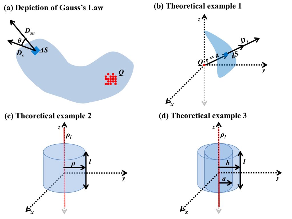
Let’s take an example of charges Q, enclosed in a closed surface of an arbitrary shape as shown in Fig. 1(a). As the charge enclosed by this surface is Q coulombs, it will also have Q coulombs of flux as well, from our previous understanding. If we take an infinitely small surface area ΔS on this surface (represented by darker blue shade on Fig. 1(a)), the ΔS will be a vector quantity of a plane surface since it will be defined by a specific place and is infinitely small. Moreover, the vector of flux density (D) will have a value of D_s, and this value will change from point to point. The surface ΔS has a unique direction, which is normal to each specific ΔS. Therefore, in mathematical form, the flux from ΔS can be defined as follows.

\[\psi=D_{sn}\Delta S=D_{s}\cos\theta\Delta S\] \[\psi=\overrightarrow{D_s} . \overrightarrow{\Delta S}\]

Therefore, the total flux passing through any closed surface will be an integral of D from all such infinitely small segments of that surface.

\[\psi=\int d\psi=\oint_{closed\hspace{0.1cm}surface} \overrightarrow{D_s} . \overrightarrow{d S}\]

The circle on the integral represents that this integral is applicable to a surface, which is a closed one. Consequently, only one integral with o means it is applicable to a surface and will be requiring two integrals. Since flux is equal to the enclosed charge we can write the following expression (Eq. 1).

\[\psi=\int d\psi=\oint_S \overrightarrow{D_s} . \overrightarrow{d S}=Q\hspace{1cm}(1)\]

The charge in the aforementioned expression can be anything, either a point charge, line charge, surface (sheet) charge, or volume charge. For all of these charge distributions, we can write an expression for Q.

\[Q=\sum Q_{charges}\] \[Q=\int\rho_l dl\] \[Q=\int_S\rho_s dS\] \[Q=\int_{vol}\rho_v dv\]

For generalization, we can take volume charge distribution, and substitute the value of Q in Eq. 1.

\[\oint_S \overrightarrow{D_s} . \overrightarrow{d S}=\int_{vol}\rho_v dv\hspace{1cm}(1)\]

We can find the charge enclosed in a sphere by considering Fig. 1(b). The flux density from a darker blue surface will be given by following.

\[\overrightarrow{D}=\frac{Q}{4\pi r^2}\overrightarrow{a_r}\]

At r=a,

\[\overrightarrow{D_s}=\frac{Q}{4\pi a^2}\overrightarrow{a_r}\]

The surface of a sphere for r=a is,

\[\overrightarrow{dS}=a^2\sin\theta d\theta d\phi\] \[\overrightarrow{D_s}\overrightarrow{dS}=\frac{Q}{4\pi a^2}a^2\sin\theta d\theta d\phi\overrightarrow{a_r}.\overrightarrow{a_r}\] \[\overrightarrow{D_s}\overrightarrow{dS}=\frac{Q}{4\pi}\sin\theta d\theta d\phi\] \[\oint_S\overrightarrow{D_s}\overrightarrow{dS}=\frac{Q}{4\pi}\int_{\phi=0}^{2\pi}\int_{\theta=0}^{\pi}\sin\theta d\theta d\phi\] \[\oint_S\overrightarrow{D_s}\overrightarrow{dS}=\frac{Q}{4\pi}\int_{\phi=0}^{2\pi} 2d\phi=Q\]

Now let’s find the charge enclosed in a cylinder having a height from z=0 to z=l as shown in Fig. 1(c). The flux density from the cylinder would be radially outwards and D would be D_ρa_ρ. We first find the Q enclosed in the cylinder.

\[Q=\oint_S \overrightarrow{D_s}.d\overrightarrow{S}=D_s\int_{lateral}dS+0\int_{top}dS+0\int_{bottom}dS\] \[=D_s\int_{z=0}^l \int_{\phi=0}^{2\pi} \rho d\phi dz\] \[=D_s2\pi \rho l\] \[D_s=D_{\rho}=\frac{Q}{2\pi \rho l}\]

If we take Q=ρ_ll we can have the same formula for electric flux density as for this case as we get with Coulomb’s law.

\[D_{\rho}=\frac{\rho_l l}{2\pi \rho l}=\frac{\rho_l}{2\pi \rho}\]

Now if we take two concentric cylinders, where the radius (ρ) of the inner cylinder is ρ=a and the radius of the outer cylinder is ρ=b and are extended to infinity. The outer surface of the cylinder with radius a has a charge of ρ_s (as shown in Fig. 1(d)). From our previous discussion,

\[Q=D_s2\pi \rho l\]

and the total charge can be calculated as,

\[Q=\int_{z=0}^l\int_{\phi}^{2\pi}\rho_s a d\phi dz \] \[= 2\pi a l \rho_s\]

and when we equate two charge distributions, we have,

\[D_s=\frac{a \rho_s}{\rho}\] \[\Rightarrow\overrightarrow{D_s}=\frac{a \rho_s}{\rho}\overrightarrow{a_{\rho}}\] \[\rho_s=\frac{\rho_l}{2\pi a}\] \[\overrightarrow{D_s}=\frac{\rho_l}{2\pi\rho}\overrightarrow{a_{\rho}}\]

The two concentric cylinder problem is an example of a coaxial cable. Here, if the outer surface of the inner cylinder has a charge of 2πaρl, the inner surface of the outer cylinder will have a charge of -2πaρl. This leads to the conclusion that the outer surface of the outer cylinder will have no charge enclosed as there are cylinders with equal and opposite charges present inside. Similarly, there will be no charge in the inner surface of the inner cylinder.

Application of Gauss’s law

As an application of Gauss’s law, we can calculate the charge enclosed in a cube in the cartesian coordinate system. A cube has 6 faces, which we will denote by front, back, left, right, top and bottom.

\[\oint_S\overrightarrow{D_s}.d\overrightarrow{S}=\int_{front}+\int_{back}+\int_{left}+\int_{right}+\int_{top}+\int_{bottom}\]

The front side will lie on the y-axis and z-axis and it’s normal to the surface area will lie on the x-axis.

\[\int_{front}=\overrightarrow{D_{front}}.\Delta S_{front}\] \[\int_{front}={D_{x-front}}\Delta y\Delta z\]

we can calculate the electric flux density by considering it as the rate of change of electric flux as the volume cube gets infinitely small, with D_xo representing the initial flux density. The electric flux density can be found from the formula below where ∂D_x/∂x represents the rate of change of D_x with respect to x.

\[D_{x-front}=D_{xo}+\frac{\Delta x}{2}\times \frac{\partial D_x}{\partial x}\Delta y \Delta z\]

Similarly, for backside,

\[D_{x-back}=-D_{xo}+\frac{\Delta x}{2}\times \frac{\partial D_x}{\partial x}\Delta y \Delta z\]

combining D_x-front and D_x-back,

\[D_{x}=\frac{\partial D_x}{\partial x}\Delta x \Delta y \Delta z\]

Similarly, we can calculate the charge enclosed for all the other sides.

\[\oint_S\overrightarrow{D_s}.d\overrightarrow{S}=\left( \begin{array}{c} \frac{\partial D_x}{\partial x} +\frac{\partial D_y}{\partial y}+\frac{\partial D_z}{\partial z}\end{array} \right)\Delta x \Delta y \Delta z\] \[\oint_S\overrightarrow{D_s}.d\overrightarrow{S}=\left( \begin{array}{c} \frac{\partial D_x}{\partial x} +\frac{\partial D_y}{\partial y}+\frac{\partial D_z}{\partial z}\end{array} \right)\Delta v\]

Therefore, the charge enclosed in a volume is given by Eq. 2.

\[Q=\left( \begin{array}{c} \frac{\partial D_x}{\partial x} +\frac{\partial D_y}{\partial y}+\frac{\partial D_z}{\partial z}\end{array} \right)\Delta v\] \[\left( \begin{array}{c} \frac{\partial D_x}{\partial x} +\frac{\partial D_y}{\partial y}+\frac{\partial D_z}{\partial z}\end{array} \right)=\frac{Q}{\Delta v}=\rho_v\hspace{1cm}(2)\]

Divergence

The divergence in terms of electric flux density is the flux from a unit volume as the volume goes to zero. The divergence is a vector operator that operates on vectors but produces a scalar quantity. The divergence of a vector field relates to the extent of that vector field behaving like a source with its flux flowing outward from an infinitely small volume. The divergence is written by div and it is a dot product of vector field with nabla (or del operator). The Eq. 2 can be written as the divergence of D.

\[div \overrightarrow{D}=\nabla.\overrightarrow{D}=\left( \begin{array}{c} \frac{\partial D_x}{\partial x} +\frac{\partial D_y}{\partial y}+\frac{\partial D_z}{\partial z}\end{array} \right)=\rho_v\hspace{1cm}(3)\]

The Eq. 3 represents the first equation of Maxwell which is derived from Gauss’s law. As we move further down our discussion we will discuss other Maxwell’s equations that form the basis of electromagnetics. The Eq. 3 can be simply written as Eq. 4 (The Maxwell’s equation of Gauss’s law).

\[\nabla.\overrightarrow{D}=\rho_v\hspace{1cm}(4)\]

for other coordinate systems, the divergence of D can be written as follows (for cylinderical and spherical coordinate systems). For cylinderical coordinate system.

\[\nabla.\overrightarrow{D}=\frac{1}{\rho}\frac{\partial}{\partial \rho}(\rho D_{\rho})+\frac{1}{\rho}\frac{\partial D_{\phi}}{\partial \phi}+\frac{\partial D_{z}}{\partial z}\]

For spherical coordinate system.

\[\nabla.\overrightarrow{D}=\frac{1}{r^2}\frac{\partial}{\partial r}(r^2 D_r)+\frac{1}{r\sin\theta}\frac{\partial}{\partial \theta}(\sin\theta D_{\theta})+\frac{1}{r\sin\theta}\frac{\partial D_{\phi}}{\partial {\phi}}\]

The divergence has units of C/m3 since it is the charge per unit volume.

Example 1

We have an electric flux density D=3r²a_r nC/m², and we need to find

a) Electric field intensity at r=3,

b) Total charge enclosed by sphere of radius r=4, and

c) Total electric flux leaving the sphere of radius r=6.

a) We have relation

\[\overrightarrow{E}=\frac{\overrightarrow{D}}{\epsilon_o}\overrightarrow{a_r}=\frac{3000\times9}{8.85}\overrightarrow{a_r}\] \[=3050.85\hspace{0.1cm}V/m\]

b) We have,

\[Q=\overrightarrow{D}\times4\pi r^2=3\times 16\times 36\pi\] \[=5428.67\hspace{0.1cm} nC\]

c) Similarly, as (b),

\[\psi=\overrightarrow{D}\times4\pi r^2=3\times 36\times 144\pi\] \[=48858.05\hspace{0.1cm} nC\]

Example 3

We need to find divergence at (1,2,3) if D=3e^-xcos(y)a_x-3e^-xsin(y)a_y+5za_z.

\[\nabla.\overrightarrow{D}=\left (\begin{array}{c} \frac{\partial (3e^{-x}\cos(y))}{\partial x} +\frac{\partial (-3e^{-x}\sin(y))}{\partial y}+\frac{\partial 5z}{\partial z}\end{array} \right)\] \[\nabla.\overrightarrow{D}=-3e^{-x}\cos(y)+3e^{-x}\cos(y)+5=5\]

Gauss’s Law

Application of Gauss’s law

Divergence

Example 1

Example 3

Further readings

Leave a Reply Cancel Reply